
The IS-LM-BP model (also known as IS-LM-BoP or Mundell-Fleming model) is an extension of the IS-LM model , which was formulated by the economists Robert Mundell and Marcus Fleming , who made almost simultaneously an analysis of open economies in the 60s. Basically we could say that the Mundell-Fleming model is a version of the IS-LM model for an open economy. In addition to the balance in goods and financial markets, the model incorporates an analysis of the balance of payments .
Even though both economists researched about the same topic, at about the same time, both have different analyses. Mundell’s paper “Capital Mobility and Stabilization Policy under Fixed and Flexible Exchange Rates”, 1963, analyses the case of perfect mobility of capital , while Fleming´s model, depicted in his article “Domestic Financial Policies under Fixed and under Floating Exchange Rates”, 1962, was more realistic as it assumed imperfect capital mobility, and thus made this one a more rigorous and comprehensive model. However, nowadays, his model has lost cogency, as the actual world situation has more resemblance with total capital mobility, which corresponds better to Mundell’s view.
In order to understand how this model works, we’ll first see how the IS curve, which represents the equilibrium in the goods market, is defined. Secondly, the LM curve, which represents the equilibrium in the money market. Thirdly, the BP curve, which represents the equilibrium of the balance of payments. Finally, we’ll analyse how the equilibrium is reached.
IS curve: the market for goods and services
In an open economy, the equilibrium condition in the market for goods is that production (Y), is equal to the demand for goods, which is the sum of consumption , investment , public spending and net exports . This relationship is called IS. If we define consumption (C) as C = C(Y-T) where T corresponds to taxes, the equilibrium would be given by:
Y = C(Y-T) + I + G + NX
We consider that investment is not constant, and we see that it depends mainly on two factors: the level of sales and interest rates. If the sales of a firm increase, it will need to invest in new production plants to raise production ; it is a positive relation. With regard to interest rates, the higher they are, the more expensive investments are, so that the relationship between interest rates and investment is negative. Now, in addition to what we have in the IS-LM model, since we have net exports, we have also to take into account the exchange rates, which directly affect net exports. Let’s say e is the domestic price of foreign currency or, in other words, how many units of our own currency have to be given up to receive 1 unit of the foreign currency. The new relationship is expressed as follows (where i is the interest rate):
Y = C (Y- T) + I (Y, i) + G + NX(e)
If we keep in mind the equivalence between production and demand, which determines the equilibrium in the market for goods, and observe the effect of interest rates, we obtain the IS curve. This curve represents the value of equilibrium for any interest rate.
An increasing interest rate will cause a reduction in production through its effect on investment. Therefore, the curve has a negative slope. The adjacent graph shows this relationship.
As stated before, we also need to analyse changes in exchange rates (here, e). If e decreases, then we’ll be able to buy more foreign currency with less of our own currency. On the other hand, foreigners we’ll need to pay more of their currency to buy our own. Therefore, when e decreases, also called an appreciation under flexible exchange rates or a revaluation under fixed exchange rates, domestic residents have more purchasing power, thus being able to buy the same amount of goods using less domestic currency. The opposite works in the same way: if e increases (also called a depreciation under flexible exchange rates or a devaluation under fixed exchange rates), domestic residents will pay more for the same goods. To sum up, an increase in e causes net exports to increase (IS curve shifts to the right) and a decrease in e causes net export to decrease (IS curve shifts to the left).
LM curve: the market for money
The LM curve represents the relationship between liquidity and money. In an open economy, the interest rate is determined by the equilibrium of supply and demand for money: M/P=L(i,Y) considering M the amount of money offered, Y real income and i real interest rate, being L the demand for money, which is function of i and Y. Also, the exchange rate must be analysed since it affects money demand (investors may decide buy or sell bonds in a country depending on the exchange rate).

The equilibrium of the money market implies that, given the amount of money, the interest rate is an increasing function of the output level. When output increases, the demand for money raises, but, as we have said, the money supply is given. Therefore, the interest rate should rise until the opposite effects acting on the demand for money are cancelled, people will demand more money because of higher income and less due to rising interest rates.
The slope of the curve is positive, contrary to what happened in the IS curve. This is because the slope reflects the positive relationship between output and interest rates.
BP curve: the balance of payments

The BP curve shows at which points the balance of payments is at equilibrium. In other words, it shows combinations of production and interest rates that guarantee that the balance of payments is viably financed, which means that the volume of net exports that affect total production must be consistent with the volume of net capital outflows . It will usually slope up since the higher the production, the higher the imports, which will disturb the equilibrium of the balance of payments, unless interest rates rise (which would cause capital inflows to maintain the equilibrium). However, depending in how great the mobility of capital is, it will have a greater or smaller slope: the higher the mobility, the flatter the curve.
Once the BP curve is derived, there is an important thing to know about how to use it. Any point above the BP curve will mean a balance of payments surplus. Any points below the BP curve will mean a balance of payments deficit. This is important since depending where we are, different things may affect the interest rates.
The IS-LM-BP model
In the model we distinguish between perfect and imperfect capital mobility, but also between fixed and flexible exchange rates. For each of these cases, we’ll see what happens when both an expansionary monetary and fiscal policy are applied to the economy. We’ll first review Mundell’s model, which deals with perfect mobility. Then, we’ll analyse Fleming’s imperfect mobility model.
1 Perfect capital mobility
1.1 Fixed exchange rate

An expansionary monetary policy will shift the LM curve to LM’, which makes the equilibrium go from point E0 to E1. However, since we are below the BP curve, we know the economy has a balance of payments deficit. Since exchange rates are fixed, government intervention is required: the government will purchase domestic currency and sell foreign currency, which will drop the money supply and therefore shift the LM’ curve to its original position (which makes the equilibrium go to E2). Monetary policy has therefore no effect under these circumstances.

An expansionary fiscal policy will shift the IS curve to IS’, moving the equilibrium form point E0 to point E1. Since the economy has now a balance of payments surplus, and because the exchange rate is fixed, government will intervene in the exact opposite way: they’ll purchase foreign currency and sell domestic currency. This will increase the money supply, shifting the LM curve to the right. The final equilibrium is reached at point E2 where, at the same interest rate, production has increased greatly: fiscal policy works perfectly under these circumstances.
1.2 Flexible exchange rate

An expansionary monetary policy will shift the LM curve to LM’, which makes the equilibrium go from point E0 to E1. However, since now exchange rates are flexible, we have a different situation: the balance of payments deficit will depreciate the domestic currency. This will increase net exports (since foreigners can now buy more of our products with the same amount of money), which will shift the IS curve to the right (to IS’). The final equilibrium is reached at point E2 where, at the same interest rate, production has increased greatly: monetary policy works perfectly under these circumstances.

An expansionary fiscal policy will shift the IS curve to IS’, moving the equilibrium from point E0 to point E1. The economy will therefore have a balance of payments surplus, which in this case of flexible exchange rate will appreciate the domestic currency. This will decrease net exports, since we are able to import more goods and services with less money, while foreigners will import less of our products because of our appreciated domestic currency. This drop in net exports will shift the IS’ curve back to its original position. Since now the final equilibrium E2 corresponds to the initial equilibrium, we know fiscal policy is no good in this case.
It is easy to see why Mundell devised what is known as the impossible trinity. In a few words, no economy can have the following three: perfect capital mobility, fixed exchange rates and an independent and efficient monetary policy. Under the perfect capital mobility assumption, and in order to have an efficient monetary policy, exchange rates must be flexible. Or have fixed exchange rates but assume that monetary policy won’t be efficient.
2 Imperfect capital mobility
2.1 Fixed exchange rate

Here we have the exact same situation as before: an expansionary monetary policy will shift the LM curve to LM’, which makes the equilibrium go from point E0 to E1. However, since we are below the BP curve, we know the economy has a balance of payments deficit. Since exchange rates are fixed, the government will purchase domestic currency and sell foreign currency, which will drop the money supply and therefore shift the LM’ curve to its original position (which makes the equilibrium go to E2). Monetary policy has again no effect, no matter how great or small capital mobility is.

An expansionary fiscal policy will shift the IS curve to IS’, moving the equilibrium from point E0 to point E1. Now, depending on capital mobility, we’ll either have a balance of payments surplus (high capital mobility, BP+ curve) or a balance of payments deficit (small capital mobility, BP- curve). Since exchange rates are fixed, government will need to intervene: its acquisitions and disposals of both domestic and foreign currency will shift the LM curve to either LM’ or to LM* (you can review what happens above: a balance of payments surplus is the same scenario as in a fiscal policy with perfect capital mobility and fixed exchange rates, while the balance of payments deficit corresponds to the monetary policy scenario). Under these circumstances, fiscal policy is completely efficient. It’s actually the more efficient the higher capital mobility is.
2.2 Flexible exchange rate

An expansionary monetary policy will shift the LM curve to LM’, which makes the equilibrium go from point E0 to E1. However, since now exchange rates are flexible, the balance of payments deficit will depreciate the domestic currency. This will increase net exports, shifting the IS curve to IS’. Also, since domestic assets are less expensive, the BP curve will shift to the right (to either BP’+ or BP’-). Therefore, with high capital mobility, final equilibrium will be at point E2. Monetary policy works well under these assumptions. It’s actually the more efficient the higher capital mobility is.
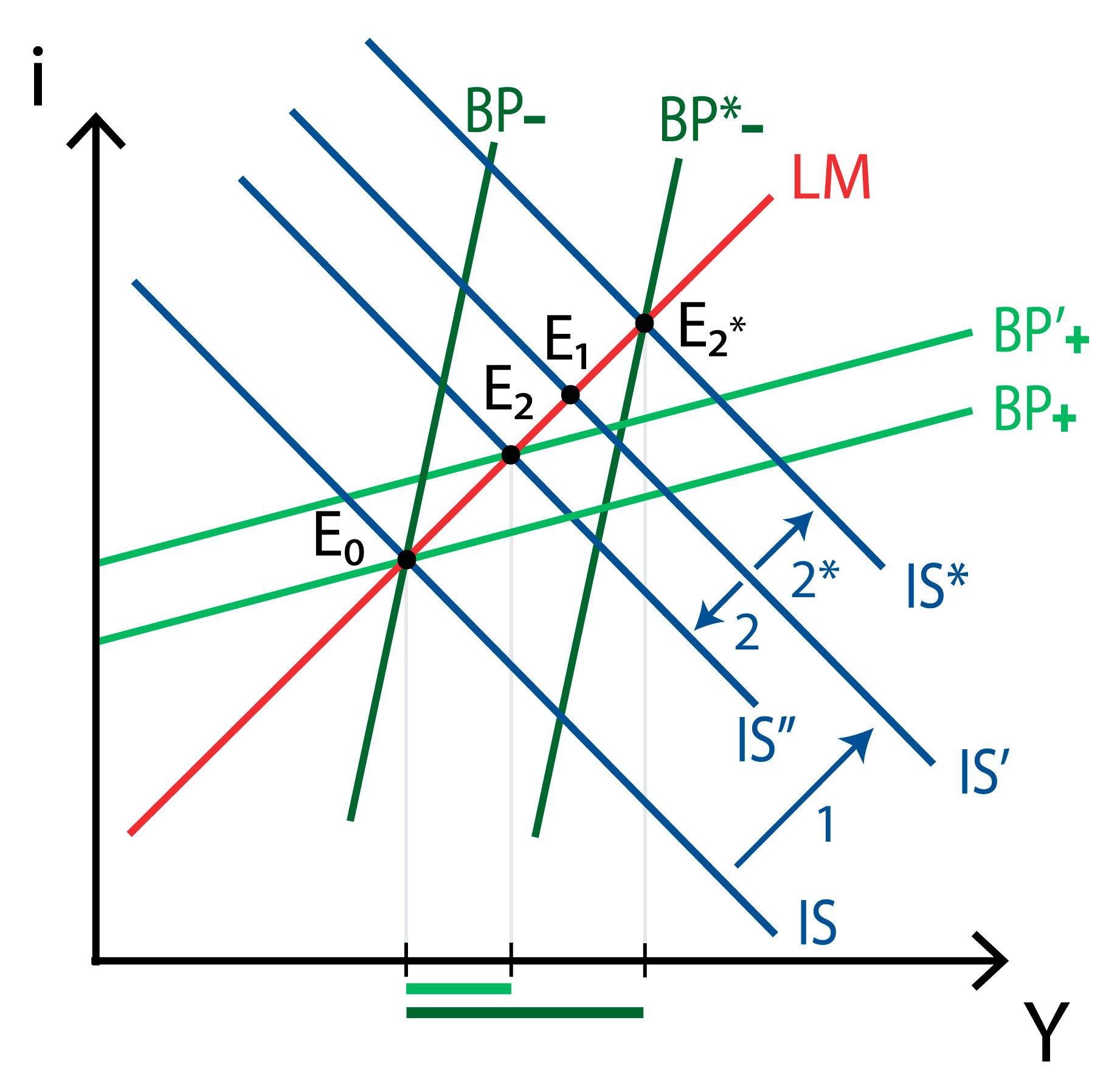
An expansionary fiscal policy will shift the IS curve to IS’, moving the equilibrium from point E0 to point E1. Now, depending on capital mobility, we’ll either have a balance of payments surplus (high capital mobility, BP+ curve) or a balance of payments deficit (small capital mobility, BP- curve). In the case of a balance of payments surplus, and considering flexible exchange rates, there will be an appreciation of the domestic currency. This will decrease net exports, which will shift the IS’ curve to the left. Also, since domestic assets are more expensive, the BP+ curve will shift to the left. The final equilibrium will therefore be at point E2. If there is a balance of payments deficit (the case for the BP- curve), the result will be the same one as in the monetary policy case (being E2* the final equilibrium). In this scenario, fiscal policy will be more efficient the smaller capital mobility is.
The Mundell-Fleming model is a very useful tool when dealing with the analysis of open economies. A great deal of textbooks and papers argue for or against each of these models. However, there’s no denying the world is moving towards liberalizing international trade and capital movements (mostly through WTO’s agreements), which would make us lean towards Mundell’s view. To sum up, under perfect capital mobility, monetary policy will only work with flexible exchange rates, while fiscal policy will only work with fixed exchange rates.